Remove solid color, gradients, or patterns from the cells in Excel 2007

To remove the solid color or gradient fill or the patterns that had been applied to the cells, you have to select the cells for which you need to remove. Once it is done, on the Home tab, in the Font group, click the down arrow in the Fill Color command (It has a paint bucket icon in it), and click No Fill.

Applying gradient fill to cells in Excel 2007

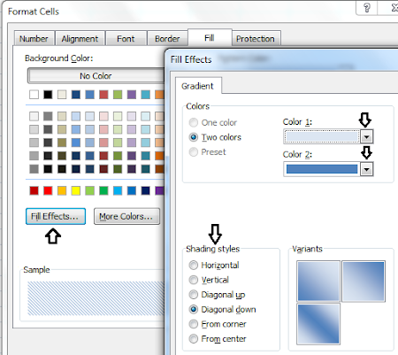
The gradient fill changes from one color to another. In short, you have two colors applied to the background. The distribution of the colors depends on the option that you choose. Perform the following steps to apply gradient fill to cells:
1. Select a cell or a range of cells. To select multiple cells, click here.
2. On the Home tab, in the Font group, click the Font dialog box launcher.
3. In the Format Cells dialog box, click the Fill tab.
4. Click Fill Effects... button to open the Fill Effects dialog box.
5. Under Color 1: click the dropdown box to pick a color.
6. Under Color 2: click the dropdown box to pick a color.
7. Choose the shading styles by clicking any one of the options available in the Shading styles group. View the sample.
8. Click OK twice.

Adding patterns to cells in Excel 2007

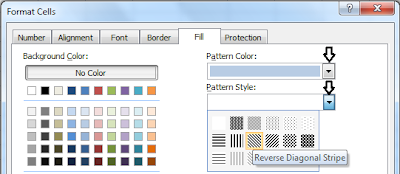
In addition to changing background color to the cells, you can add decoration to the cells by adding patterns to the cells. Perform the following steps to add patterns to the cells:
1. Select a cell or a range of cells. To select multiple cells, click here.
2. On the Home tab, in the Font group, click the Font dialog box launcher.
3. In the Format Cells dialog box, click the Fill tab.
4. Under Pattern Color: click the dropdown box and click to select a color.
5. Under Pattern Style: click the dropdown box and click to select a pattern.
6. Click OK.

Change the background color of cells in Excel 2007

To change the background color of the cells, select an individual cell or select multiple cells first. Click here for information regarding selecting multiple cells.

On the Home tab, in the Font group, click the arrow next to the Fill Color command (It has the paint bucket icon in it). Click to apply that color as the background color for the cell(s).

If the color that you are looking for is not available under Theme Colors or Standard Colors then click More Colors... to open the Color dialog box. Pick a color from the Standard tab or from the Custom tab and click OK.
In the figure to the right, few cells in column C and D are selected and applied Purple, Accent 4, Lighter 40% color.

Change the color of text in Excel 2007

In Excel, the default color when you type text is black. At times, you need to add customization so that some information appears with a different color. This will give good attention to the parts of the sheet that holds critical information or a better look. To change the color of the text, on the Home tab, in the Font group, click the down arrow in the Font Color button and select a color.

Underlining text in Excel 2007

There are several ways to underline text. You can use the Underline command to underline the text in the cell(s) (or) apply the border bottom style to cell(s) (or) draw a line just below the text. You can also add a double underline to the text or to the entire cell(s). We will discuss all the ways in detail:

Single underline only the text:
On the Home tab, in the Font group, click the Underline command.

Double underline only the text:
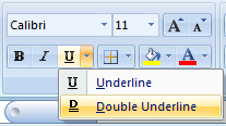
On the Home tab, in the Font group, click the down arrow in the Underline command and click Double Underline.

Single underline the entire cell or multiple cells - Single Accounting:
1. On the Home tab, in the Font group, click the dialog box launcher (a small arrow in the right corner) to open Format Cells dialog box.
2. Click the Font tab, click the Underline: dropdown box and click Single Accounting.
3. Click OK.

Double underline the entire cell or multiple cells - Double Accounting:
1. On the Home tab, in the Font group, click the dialog box launcher (a small arrow in the right corner) to open Format Cells dialog box.
2. Click the Font tab, click the Underline: dropdown box and click Double Accounting.
3. Click OK.

Apply the border bottom style to give an underline effect:
Click the cell. On the Home tab, in the Font group, click the down arrow in the Border command that is to the right of the Underline command. You can apply the borders by clicking one of the following:
Bottom Border, Bottom Double Border, Thick Double Border
For more styles, click More Borders and select a border style from the Style: box. In the Border click the bottom line and click OK.

Draw line to give an underline effect:
Click Insert tab, in the Illustrations group, click Shapes. In the Lines section, click the first option (It is a diagonal line).
The cursor changes to a plus sign. Draw the line just below the text for which you need to apply the underline effect.

Apply Bold, Italics, or Underlines to cells in Excel 2007

By default when you enter text in a cell, the text is not bold, no italic style or underline style is applied. You can apply the style to selected text or to the entire cell or to multiple cells. To make the text bold, click the Bold command on the Home tab (or press CTRL + B). For displaying the text in italic style, click the Italic command (or press CTRL + I). For underlining selected text, click the Underline command (or press CTRL + U).

You can have any or all the three styles applied to the selected text, to the cell, or to multiple cells. For example, the selected text can be bold, italic, and underlined (or) bold and italic.

Note:
You have more options for underlining cell contents and is described in a separate post. Click here to see the post "Underlining text in Excel 2007".

Bold Italic and Underline commands grayed out in Excel 2007

In the worksheet, if you see the Bold, Italic, Underline, and other commands grayed out then the worksheet would be protected and during protecting, the Format cells check box might have the checkbox cleared in the Allow all users in this worksheet to: section. Unprotect the worksheet by clicking the Review tab, in the Changes group click Unprotect Sheet. If any password is applied then enter the password to unprotect the worksheet.

Change the font size for cells in Excel 2007

By default, in Excel 2007 the Calibri font of size 11 point. The size of the font is represented by points. You can change the font size and apply different sizes for individual cells and also apply different sizes for some text in a single cell.
On the Home tab, in the Font group, when you click on the Font Size dropdown box, you will see the points 8, 9, 10, 11, 12, 14, 16, 18, 20, 22, 24, 26, 28, 36, 48, and 72. If you see outside of these entries then it is particular for that font.
Now the tricky part, how do you have font size outside of the entries provided above? The answer is, in the Font Size box type the size of the font. You can also enter .5 incremental values for the font size. For example, font size 22.5 is acceptable but entering other values like 22.8 or 22.1 is not acceptable.

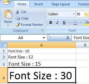
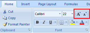
You can also increase or decrease the size of the font by clicking on the Increase Font Size or Decrease Font Size commands. The font size will increase according to the values provided above. For example, if the current font size is 28 and you click the Increase Font Size then the size will change to 36.

Change the font for cells in Excel 2007

By default, in Excel 2007 the Calibri font is applied for all cells. You can change this default setting and apply different font for individual cells. For example, cell A1 can have the font Arial, cell A2 can have the font Courier, and cell A3 can have the font Verdana. You apply the font to a cell from the Font group that is on the Home tab and clicking the Font dropdown box and making a font selection.

You can also have a cell formatted with multiple fonts. For example in cell A4, you type Arial Courier Verdana. Highlight Arial and from the Font group, select the font Arial from the Font dropdown box. Highlight the text Courier and select the font Courier. Highlight the text Verdana and apply the font Verdana.

Transpose data in Excel 2007

At times, you might had entered some data in rows and later realize that it should had been entered in columns. You can move the data in the rows to columns and vice versa. This is called transpose. To perform transpose of data, do the following:
1. Select the cells that you need to transpose.
2. On the Home tab, in the Clipboard group, click Copy.

3. Click cell A2 or the cell where you need to have the data.
4. On the Home tab, in the Clipboard group, click the down arrow in the Paste command and click Transpose.

Output: