Difference between Erase Border and No Border in Excel 2007

The Erase Border and No Border erase the border with the difference being the way they remove the border.
In Erase Border, you do not have to select the range of cells to remove the borders. You have to drag the mouse to perform the removal of borders or click on a border side to remove the border. In No Border, you have to select the range of cells and then perform the removal of borders.
In Erase Border, the least that you can remove is a border side, i.e., either Top Border, Right Border, Bottom Border or Left Border. In No Border, the least that you can remove is the borders around 1 cell.

Create a custom cell border in Excel 2007

You can create your own cell border and apply to the cells. Perform the following steps to create a custom border:

1. On the Home tab, in the Styles group, click Cell Styles and click New Cell Style...
2. In the Style dialog box, in the Style name: box, type a name for the new cell style.
3. Click Format... button.

4. In the Format Cells dialog box, click the Border tab and do the following that suits your needs:
    a. Under Style: click to select a style.
    b. Under Color: click to select a color for the border.
    c. Under Border, click the sides of the border to apply the border.
    d. Click OK to close the Format Cells dialog box.

5. Click OK to close the Style dialog box.

To apply the custom border to cells, perform the following:
1. Select the cells for which you need to apply the custom border.
2. On the Home tab, in the Styles group, click Cell Styles. Under Custom, the created styles appear. Click on the cell style that you need to apply.

Keyboard shortcut for applying border to cells in Excel 2007

After selecting a cell or a range of cells and clicking the Font dialog box launcher. In the Border tab of the Format Cells dialog box, you will see 8 buttons under Border. When you click on a button, the color of the button changes to blue. This means the border is applied. When you click the same button again, the border gets removed. You can access these 8 buttons through keyboard also. The keyboard shortcut is shown below:

    Top Border                                ALT + T

    Horizontal Interior Border         ALT + H 

    Bottom Border                          ALT + B 

    Upward Diagonal Border          ALT + U

    Left Border                               ALT + L

    Vertical Interior Border            ALT + V

    Right Border                            ALT + R 

    Downward Diagonal Border    ALT + D 

Apply diagonal border for cells in Excel 2007

If you have worked on borders, you will know that you apply borders to all the sides of the cell(s) but for most of them they do not know that there is few more options available while it comes to drawing borders. You can draw borders that is dialgonally left across the cell(s) or diagonally right across the cell(s). To apply diagonal border to the cells, perform the following:

1. Select a cell or a range of cells. To select multiple cells, click here.
2. On the Home tab, in the Font group, click the Font dialog box launcher.
3. In the Format Cells dialog box, click the Border tab.
4. Under Border, click the buttons that has the diagonal line to draw diagonal borders.
5. Click OK.

Difference between Draw Border Grid and All Borders in Excel 2007

The Draw Border Grid and All Borders do the same function. They both draw the inside and outer border for the cells. The difference is in how they do it. In the All Borders, you select the cells and draw the border. In Draw Border Grid, you drag across the cells and when you release the mouse, the borders is drawn. You can access the Draw Border Grid and All Borders by clicking on the Home tab, in the Font group, click the DOWN arrow in Borders command and clicking Draw Border Grid or All Borders. We will see each of them individually so that it will be easy to understand.

All Borders: You have to highlight the cells for which you need to apply the outer border. Once the cells are selected, on the Home tab, in the Font group, click the DOWN arrow in Borders command and click All Borders.

Draw Border Grid: On the Home tab, in the Font group, click the DOWN arrow in Borders command and click Draw Border Grid. The mouse cursor will turn into a pen and a small square. Click and drag across the cells to draw the borders.

Difference between Draw Border and Outline Borders in Excel 2007

The Draw Border and Outline Borders do the same function. They both draw an outer border around the cells. The difference is in how they do it. In the Outline Border, you select the cells and draw the border. In Draw Border, you drag across the cells and when you release the mouse, the border is drawn around the cells. You can access the Draw Border and Outline Borders by clicking on the Home tab, in the Font group, click the DOWN arrow in Borders command and clicking Draw Border or Outline Borders. We will see each of them individually so that it will be easy to understand.

Outline Borders: You have to highlight the cells for which you need to apply the outer border. Once the cells are selected, on the Home tab, in the Font group, click the DOWN arrow in Borders command and click Outline Borders.

Draw Border: On the Home tab, in the Font group, click the DOWN arrow in Borders command and click Draw Border. The mouse cursor will turn into a pen. Click and drag across the cells to draw an outline border.

Remove borders around cells in Excel 2007

To remove border around cells, highlight the cells for which you need to remove the border. Once you had highlighted the cells, on the Home tab, in the Font group, click the arrow next to Borders and then click No Border

You can also remove the borders around the cells by performing the following:

1. Select the cells that need the borders to be removed.
2. On the Home tab, in the Styles group, click Cell Styles. Under Good, Bad and Neutral, click Normal.

Change border style in Excel 2007

You can change the border style directly from the Ribbon or from the Format Cells dialog box. We will see the two ways for changing the border style for cell(s).

Change the border style from the Ribbon:
1. On the Home tab, in the Font group click the DOWN arrow in Borders and point to Line Style. Click to select a style.
2. The mouse cursor changes to a Pen. Press the Esc key.
3. Select the cell(s) for which you need to change the border style. For selecting multiple cells, click here.
4. On the Home tab, in the Font group click the DOWN arrow in Borders and click All Borders.

Change the border style from the Format Cells dialog box:
1. Select the cell(s) for which you need to apply the border style. For selecting multiple cells, click here.
2. Press CTRL + 1 to open Format Cells dialog box.
3. Click the Border tab.
4. Click on a style under Style: box.
5. Under Presets, click Outline and also click Inside.
6. Click OK.

Change border color in Excel 2007

By default black color border is applied to cells. You can change the border color directly from the Ribbon or from the Format Cells dialog box. We will see the two ways for changing the border color for cell(s).

Change the border color from the Ribbon:
1. On the Home tab, in the Font group click the DOWN arrow in Borders and point to Line Color. Click to select a color. If you need to select a different color then click More Colors... to open Colors dialog box. Make a selection and click OK.
2. The mouse cursor changes to a Pen. Press the Esc key.
3. Select the cell(s) for which you need to change the border color. For selecting multiple cells, click here.
4. On the Home tab, in the Font group click the DOWN arrow in Borders and click All Borders.

Change the border color from the Format Cells dialog box:
1. Select the cell(s) for which you need to change the border color. For selecting multiple cells, click here.
2. Press CTRL + 1 to open Format Cells dialog box.
3. Click the Border tab.
4. Under Color: click the DOWN arrow button and click to select a color.
5. Under Presets, click Outline and also click Inside.
6. Click OK.

Button raised and sunken effect for cells using border color and fill color in Excel 2007

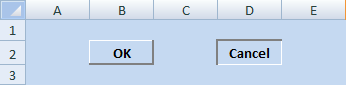When you apply proper border color and color fill to the cell, you have raised and sunken effect that appears in a button. In the figure to the right, you will see cell B2 has the raised effect and cell D2 has sunken effect. You can create this effect by performing the following:

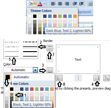1. Color the background for cells A1 to E3: Click cell A1. Press the SHIFT key. Keeping the SHIFT key in pressed state, click cell E3. On the Home tab, in the Font group, click the arrow in the Fill Color command and click Dark Blue, Text 2, Lighter 80%.
2. Apply the raised effect for cell B2: Click cell B2. Press CTRL + 1 to open Format Cells dialog box.
3. Click the Border tab and do the following:
I. Under Color: click the DOWN arrow, click Black, Text 1, Lighter 50% color. (labeled 1 in the figure).
II. Under Style: click the line as shown in the figure with the label 2.
III. Under Border, click the Bottom Border button (labeled 3) and click Right Border button (labeled 4).
IV. Under Style: click the line as shown in the figure with the label 5.
V. Under Color: click White, Background 1 (labeled 6).
VI. Under Border, click the Left Border button (labeled 7) and click Top Border button (labeled 8).
4. Click OK.

5. Apply the sunken effect for cell D2: Click cell D2. Press CTRL + 1 to open Format Cells dialog box.
6. Click the Border tab and do the following:
I. Under Color: click the DOWN arrow, click Black, Text 1, Lighter 50% color. (labeled 1 in the figure).
II. Under Style: click the line as shown in the figure with the label 2.
III. Under Border, click the Left Border button (labeled 3) and click Top Border button (labeled 4).
IV. Under Style: click the line as shown in the figure with the label 5.
V. Under Color: click White, Background 1 (labeled 6).
VI. Under Border, click the Right Border button (labeled 7) and click Bottom Border button (labeled 8).
7. Click OK.

Create 3D effect for cells in Excel 2007

You can play around with borders and apply suitable colors to the borders so that the cell appears with 3D effect. In the figure to the right, you will see two cells B2 and D2. These cells appear as buttons. You can create this effect by performing the following:

1. Color the background for cells A1 to E3: Click cell A1. Press the SHIFT key. Keeping the SHIFT key in pressed state, click cell E3. On the Home tab, in the Font group, click the arrow in the Fill Color command and click Blue, Accent1, Lighter 80%.
2. Click cell B2. Press the CTRL key. Keeping the CTRL key in pressed state, click cell D2. Click the Fill Color command and click Tan, Background 2, Darker 10% (It is second left from the Blue, Accent1, Lighter 80% color).

3. Click cell B2, press CTRL key. Keeping the CTRL key in pressed state, click cell D2. Open Format Cells dialog box by pressing CTRL + 1 (or) on the Home tab, in the Font group, click the DOWN arrow in the Borders command and click More Borders...

4. In the Format Cells dialog box, click the Border tab and do the following:
Under Style:, click the line as shown in the figure with the label 1.
Under Color:, click Automatic. It is labeled 2 in the figure.
Under Border, click the Bottom Border button (labeled 3) and click Right Border button (labeled 4).
Under Color:, click White, Background 1 (labeled 5).
Under Border, click the Left Border button (labeled 6) and click Top Border button (labeled 7).

5. Click OK.