Compare data using Row differences in Excel 2007

Using Row differences, you compare the data in a cell that belongs to a row with other cells in the same row and highlight the cells that have different data. Also, you can extend the selection area. You can select multiple rows of data and Excel will do the comparison for you automatically. An example will make you understand this feature clearly. The following figure shows the sample temperature reading for a period of 5 years with data recorded month wise.

In the figure to the right, the data in cell C4 which is 23 is compared with other cells in that row, which are 23, 23, 24, and 23. You will see the data that is different is present in cell F4. Similarly when you compare the data in C5 which is 31 with other cells in that row, you will see that the data in the cells E5 (32) and G5 (30) are different. When we do the comparison for the rest of the data, we expect Excel to highlight the cells that have different data.

Perform the following to use the Row differences feature:
1. Highlight cells C4 to G15.
2. On the Home tab, in the Editing group, click Find & Select and click Go To Special...
3. In the Go To Special dialog box, click Row differences and click OK.
4. On the Home tab, in the Font group, click the Fill Color command and pick a color.

Additional Reading:
The figure above highlighted all the cells that has data that is different from the data that is present in column C. In practical terms, you have compared the temperature of each month in 2006 with the months in other years.

To do the comparison for the year 2007 with other years. You may first try the following:
1. Highlight all the cells. On the Home tab, in the Font group, click the Fill Color command and click No Fill.
2. With the cells still highlighted. Press the TAB key. The active cell is moved to the cell D4.
3. On the Home tab, in the Editing group, click Find & Select and click Go To Special...
4. In the Go To Special dialog box, click Row differences and click OK.
5. On the Home tab, in the Font group, click the Fill Color command and pick a color.

Select named cells or ranges using the Go To command in Excel 2007

You have to name the cells or ranges in order to select named cells or ranges using the Name box. Assuming that you had already named the cells or ranges, perform the following steps:
1. Press F5 to open the Go To dialog box.
2. The Go to: list box displays all the names. Click the name and click OK.

To select multiple names, you have to perform the above steps and again press F5 to open the Go To dialog box and select a different name. Now, press and hold the CTRL key and click OK.

Select unnamed cells or ranges using the Go To command in Excel 2007

To select unnamed cells or ranges using the Go To command, do the following:
Selecting a single cell: Press F5 to open the Go To dialog box. Type the cell reference in the Reference box and click OK. For example: if you type C4 and press the ENTER key, cell C4 will be selected.
Selecting a range of cells: Press F5 to open the Go To dialog box. Type the cell reference for the range of cells in the Reference box and click OK. For example: if you type C2:C10 and press the ENTER key, cells C2 to C10 will be selected.

Select unnamed cells or ranges using the Name box in Excel 2007

To select unnamed cells or ranges using the Name box, do the following:
Selecting a single cell: Click the Name box and type the cell reference and press the ENTER key. For example: if you type B4 and press the ENTER key, cell B4 will be selected.
Selecting a range of cells: Click the Name box and type the cell reference for the range and press the ENTER key. For example: if you type C2:C10 and press the ENTER key, cells C2 to C10 will be selected.

Select named cells or ranges using the Name box in Excel 2007

You have to name the cells or ranges in order to select named cells or ranges using the Name box. Assuming that you had already named the cells or ranges, do as per in the following line:

In the Name box, click the arrow and then click the name.

Tip:

#1. To select two or more names, click the arrow in the Name box and click the name. Press and hold the CTRL key. Click the arrow in the Name box and click the other name.

#2. You can click on only one name at a time. You have to click the arrow in the Name box and click the other name and repeat doing this for the number of names that you want to select.

#3. You cannot delete a name from the Name box.

To know how to name a cell or range, click here.

Selecting blank cells in Excel 2007

To select blank cells, do the following:
1. Select a range of cells.
2. On the Home tab, in the Editing group, click Find & Select and then click Go To Special...
3. In the Go To Special dialog box, click Blanks.
4. Click OK.

Additional Reading:

• Click CTRL + END key to know the last cell that has the data in the worksheet. Excel will select all the blank cells till this region only.
• Excel will not select blank cells in an empty worksheet.

Selecting cells that contain formulas in Excel 2007

To select cells that contain formulas in the worksheet, perform the following steps:
1. On the Home tab, in the Editing group, click Find & Select and then click Go To Special...
2. In the Go To Special dialog box, click Formulas.
3. Click OK.

Note:

• You can choose the formulas that returns numbers or text or logicals or errors by placing or removing the checkmark besides Numbers, Text, Logicals, Errors.
• You can select the cells with formulas in a range of cells by selecting the cells first and performing the above steps.

Selecting cells that contain constants in Excel 2007

To select cells that contain constants in the worksheet, do the following:
On the Home tab, in the Editing group, click Find & Select and then click Constants .

Note:
You can select the cells with constants in a range of cells by selecting the cells first and performing the above steps.

Selecting cells that contain comments in Excel 2007

To select cells that contain comments in the worksheet, do the following:
On the Home tab, in the Editing group, click Find & Select and then click Comments.

Note:
You can select the cells with comments in a range of cells by selecting the cells first and performing the above steps.

How Excel selects a region?

A region is a group of cells with data and is bounded by blank cells around it (or) a block of cells that includes the currently selected cell or cells and is bounded by blank columns and rows.. To identify a region in a group of cells, click a cell and press CTRL + SHIFT + *. Press the * that is above the number 8 and not the * in the number pad.
For the sake of explanation, we will enter blank cells as well. Also, we will add data in cells as we go along:
Enter 1 in cell D3, and 1 in cell E4. Click cell D3 and press CTRL + SHIFT + *. Cells C2 to F2, C3 to C5, D5 to F5, and F3 to F4 are all blank. So, the region is D3:E4.

Add 1 in F5. Click cell D1 and press CTRL + SHIFT + *. You will see the region in the following in the following figure because the cells around, i.e., C2 to G2, C3 to C6, D6 to G6, G3 to G5 are all blank cells.

In the following figure, we add 1 in G2, 1 in D6, 1 in G7. Click cell D1 and press CTRL + SHIFT + *. You will see that G2 was blank in figure 1 but now it is not blank and so it is included in the region. Similarly, D6 is not blank now and is included in the region. With the region spanning across D2:G6, cells around D2:G6 should be blank but G7 has the data 1 and so it is included in the region. The region now spans from D2:G7.

We will add data in 3 more cells. We add 1 in cell B9, 1 in cell C8, and 1 in cell G10. From the figure above the region spanned from D2:G7. Click cell D1 and press CTRL + SHIFT + *, you will see that the region now spans from B2:G10.

Generally a region must have filled cells. The example was to show how Excel selects a region. In this example, the region was from B2:G10. If there are plenty of blank cells then it is not true that the same region will appear if you click other cells and press CTRL + SHIFT + *. For instance, try clicking B9 or B7 or D6 or any cell from B2:B6 and press CTRL + SHIFT + *.

Selecting a region in Excel 2007

A region is a group of cells with data and is bounded by blank cells around it (or) a block of cells that includes the currently selected cell or cells and is bounded by blank columns and rows. To select a region, do one of the following:

• Press CTRL + SHIFT + *. The * that is above the number 8 and not the * in the number pad.
• 1. On the Home tab, in the Editing group, click Find & Select and then click Go To Special...
  2. In the Go To Special dialog box, click Current region.
  3. Click OK.

Selecting the entire worksheet in Excel 2007

You can select the entire worksheet by clicking the grey box that is to the left of the Column heading A.

Alternative ways to select the entire worksheet:

• Press CTRL + A to select the entire worksheet.
• Press CTRL + SHIFT + SPACEBAR to select the entire worksheet.

In the alternative ways provided above, if you attempt to key in CTRL + A or CTRL + SHIFT + SPACEBAR in a region then only the cells in the region get selected. Press CTRL + A or CTRL + SHIFT + SPACEBAR again to select the entire worksheet.

You may also try this. Click cell A1 and press the CTRL + SHIFT + RIGHT arrow keys and CTRL + SHIFT + DOWN arrow keys to select the entire worksheet.

Selecting columns in Excel 2007

By default, every column looks alike. To identify the columns, Excel displays column header with letter(s). Column header appears at the top most part of the worksheet area.

Selecting a single column:
Perform any of the following to select a single column.

• To select an entire column, click on the column header.
• Click a cell that corresponds to the column. Press CTRL + SPACEBAR.
• Click the first cell in the column and press CTRL + SHIFT + DOWN arrow keys. If data is present then the selection is made till the end of the cells that contain the data. Pressing CTRL + SHIFT + DOWN arrow keys again will select the entire column provided that no data is present in between.

Selecting multiple columns:

• Select adjacent columns by clicking the column header and pressing the SHIFT key and finally clicking the column letter in the column header.
• Select nonadjacent columns by selecting the first column (click the column letter) and pressing the CTRL key and clicking other column letter(s) in the column header.

Selecting rows in Excel 2007

By default, every row looks alike. To identify the rows, Excel displays row header with numbers. Row header appear at the left most part of the worksheet area.

Selecting a single row: (Perform any one of the following)

• Click the row header.
• Click a cell that corresponds to the row. Press SHIFT + SPACEBAR.
• Click the first cell in the row and press CTRL + SHIFT + RIGHT arrow keys. If data is present then the selection is made till the end of the cells that contain the data. Press CTRL + SHIFT + RIGHT arrow keys again to select the entire row provided that no data is present in between.

Selecting multiple rows:

• You can select adjacent rows by clicking the row header and pressing the SHIFT key and clicking the last row number in the row header.
• You can select nonadjacent rows by selecting the first row (click the row number) and pressing the CTRL key and clicking other row numbers in the row header.

Selecting nonadjacent cells in Excel 2007

To select nonadjacent cells, perform any one of the following:

• Click a cell. Press and hold the CTRL key. Clicking the remaining cells.
• Click a cell. Press SHIFT and F8 keys. You will see Add to Selection in the Status bar. Click other cells. Once the selection of cells is over, press SHIFT and F8 keys.

Things you can do:
You can copy nonadjacent cells if the cells are in the same row or same column. The cells will be pasted into adjacent cells. In the image below, cells A1, C1, and E1 are copied and pasted in A3. They get pasted in cells A3, B3, and C3.

Things you cannot do:

• You cannot copy cells if the nonadjacent cells span across multiple rows and columns. You will receive the warning message saying That command cannot be used on multiple selections.
• You cannot drag and drop the cells that span across multiple rows and columns to another location.

Selecting adjacent cells in Excel 2007

Select adjacent cells by clicking a cell and dragging the mouse over a group of cells. This works good if the selection area is small. If the selection area is large then click the first cell in the selection area. Press and hold down the SHIFT key. Click the last cell to make the selection.

Alternative ways to select adjacent cells:
1. Click the first cell. Press and hold the SHIFT key. Press the RIGHT or LEFT arrow key to make the selection of cells in the row. With the SHIFT key still in pressed state, press the UP or DOWN key to make the selection of columns.
2. Click the first cell. Press the F8 key. You will see Extend Selection in the Status bar. Click the last cell in the selection area. Press F8 key again.

Things to notice when selecting adjacent cells:
1. The Name box will display the number of rows and columns selected while performing the selection process.
2. The column and row headers will be shaded to identify the selected rows and columns.
3. One cell in the selected cells is active and is highlighted in white.

Things you can do:
1. You can copy or move the data in the selected cells to another location.
2. You can enter data in the selected cells.
3. You can enter data in a cell and copy the data to all cells in the selected area.

Selecting a cell in Excel 2007

To select a cell, use any of the following techniques:
Use the mouse: Move the mouse cursor to a particular cell and click to select the cell.
Use the arrow keys in the keyboard: To move to the adjacent cells, press the UP or DOWN or LEFT or RIGHT arrow key.
Use the ENTER key in the keyboard: Press the ENTER key to select the cell that is below the current cell. This is the default setting unless an Excel option to change the direction of the ENTER key is modified.
Use the Name box on the Formula bar: In the Name box, type the cell address (Example: A4) and press the ENTER key.
Use the Go To feature: Press F5 to display the Go To dialog box. Type the cell reference in the Reference box (Example: D5) and click OK.

Things to note for identifying the selected cell:

• The selected cell is surrounded by a thick border with a small square at the lower right corner.
• The Row heading and the column heading corresponding to the cell is shaded. For example, if cell G4 is selected then column number G in the column header and row number 4 in the row header is shaded.
• The address of the selected cell is displayed in the Name box.

Select multiple cells in Excel 2007

At times, you may want to select multiple cells to apply the setting to all the cells like changing the font, applying borders, changing the background color of cells or applying other formatting details. You may also perform copy or move operations like copying or moving data in a row or range to other location or whatever the needs are. At those cases, you have to select multiple cells. We will discuss the ways of selecting multiple cells.

Selecting column(s):

• Click the column heading (e.g., A or B or C or D) to select single column.
• To select multiple columns that are adjacent: Click a column first. Press and hold the SHIFT key. Click the last column.
• To select nonadjacent columns: Click a column first. Press and hold the CTRL key. Click other columns.

Two columns (B and D) are selected by clicking the column header B, pressing the Ctrl key and clicking on the column header D.

Selecting row(s):

• Click the row number to select single row.
• To select multiple rows that are adjacent: Click a row first. Press and hold the SHIFT key. Click the last row to select.
• To select nonadjacent rows: Click a row first. Press and hold the CTRL key. Click other rows to select them.

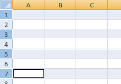
Four rows (1, 3, 5, and 7) are selected by clicking the row number 1, pressing the Ctrl key and clicking on the row numbers 3, 5, and 7.

Selecting cells that span across multiple rows and columns:
Two cases in this section.

1. Selecting cells that are adjacent across rows and columns
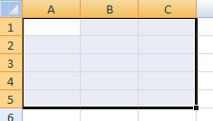
The cell selection is from A1 to C5. To make this selection, click cell A1. Press the Shift key and keep the Shift key in pressed state, click cell C5.

2. Selecting cells that are not adjacent across rows and/or columns
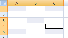
Cells A1, A5, B3, C1, C4, and C5 are selected. To make this type of selection, click cell A1. Press and keep the Ctrl key in pressed state, click cells A5, B3, C1, C4, and C5.

Selecting the entire worksheet
Press Ctrl + A (Or) click the grey box that is to the left of the Column heading A.