Rotate cell data in Excel 2007

You can rotate the cell data if the width of the cell is narrow or to make the column headers stand out from the data cells or to make the header be present by merging rows.
You can rotate the cell data clockwise, counterclockwise, vertically, and can also rotate the data with degrees precision.

To rotate cell data, select the cells first. On the Home tab, in the Alignment group, click Orientation button and click on one of the option.
To specify the number of degrees the text will be rotated, click the Format Cell Alignment option. The Format Cells dialog box dialog box opens. In Orientation, click the UP or Down arrow button in the Degrees spin box. You can also enter a number directly in the box. The allowable range of values is -90 to 90 degrees. Click OK.

Justify text alignment option in Excel 2007

With justify, the text in the cell gets distributed evenly across the cell. If the text in the cell is large then part of the text overflows to the adjacent cells. If you apply the Justify alignment then the following occurs:

• The text in the cell gets wrapped.
• The cell adjusts the row height to fit the content.

Select cells A1 to A3 and perform the following steps to apply Justify:
1. On the Home tab, in the Alignment group, click the dialog box launcher to open Format Cells dialog box.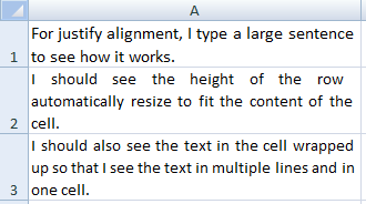
2. In Text Alignment, under Horizontal: click the dropdown box and select Justify.
3. Click OK.

Distributed indent in Excel 2007

To see what distributed indent does, enter two or more words of information in a cell. Distributed indent will enlarge the spaces between the text and also fills the entire cell.
You can add the indent levels. If you increase the indent level then the margin between the border and the text in the cell increases from left and right.

To apply distributed indent, perform the following:
1. On the Home tab, in the Alignment group, click the dialog box launcher to open the Format Cells dialog box.
2. In Text Alignment, under Horizontal: click the dropdown box and select Distributed (Indent).
3. If you need to add indent levels then under Indent, click the Up or Down arrow to increase or decrease the indent level. You can also type a number directly in the Indent box.
4. Click OK.

Indent options in Excel 2007

In Excel 2007, you have:

• Left (Indent)
• Right (Indent)
• Distributed (Indent)

You can add indent levels, which can be increased or decreased by 1. You can add the indent levels to all the three indent types. To apply the indent type, perform the following: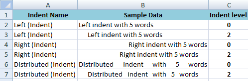
1. On the Home tab, in the Alignment group, click the dialog box launcher to open the Format Cells dialog box with focus on the Alignment tab.
2. In Text Alignment, under Horizontal: click the dropdown box and select Left (Indent) or Right (Indent) or Distributed (Indent).
3. Under Indent, click the Up or Down arrow to increase or decrease the indent level. You can also type a number directly in the Indent box.
4. Click OK.

Apply or remove indent from the Ribbon in Excel 2007

When you apply the indent, the text gets displayed away from the border of the cell. In other words, you are increasing the margin between the border and the text in the cell. To apply the indent, on the Home tab, in the Alignment group, click the Increase Indent command.
On clicking the Increase Indent command repeatedly, the text moves farther away. If the text is wrapped then the data in all the lines move at the same time.

Keyboard shortcut:
Press CTRL + ALT + TAB

Remove or decrease the indents:
On the Home tab, in the Alignment group, click the Decrease Indent command. On clicking the Decrease Indent command repeatedly reduces the indent level.

Unmerge cells in Excel 2007

You can unmerge cells only if it had already been merged. Also, you cannot unmerge a single cell (for example cell A1). If data is present in the larger cell then after unmerging, the data will be present in the first cell of the unmerged cells. For example, if cells E1, F1, G1 are merged and has data Excel 2007 Unmerge post. After the unmerge, the text will be present in the cell E1.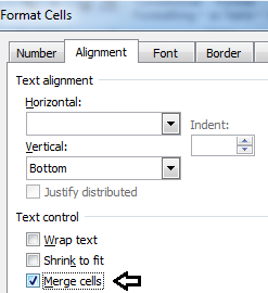

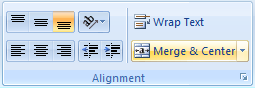
Perform the following to unmerge cells:
1. Click the merged cells.
2. On the Home tab, in the Alignment group, click the DOWN arrow in Merge & Center command and click Unmerge Cells.

Merge cells using the Format Cells dialog box in Excel 2007

You can merge cells from the Home tab in the Ribbon. You can also merge cells from the Format Cells dialog box.

Perform the following steps to merge cells from the Format Cells dialog box:
1. Select the cells that you need to merge. Click here for information regarding selecting multiple cells.
2. Press CTRL + 1 to open the Format Cells dialog box.
3. Click the Alignment tab. Under Text control, click Merge cells.
4. Click OK.

Note:
If you enter data in the merged cells, the data will be left aligned horizontally if you enter text and right aligned if you enter numbers.

Cell merge options in the Ribbon in Excel 2007

In Excel 2007, you can join the selected cells into one larger cell. There are few options available on the Ribbon for merging cells. We will discuss each option in detail here:

Merge & Center: This option will merge all the selected cells into one cell plus the data in the cell will be aligned to the center horizontally.

Merge Across: When you select cells that spans across rows and columns (for e.g., cells A1 to D5 are selected). The merge occurs across the rows i.e., cells A1 to A5 are merged as one cell. Cells B1 to B5 as one cell and so on. The default alignment of left to the text and right to the numbers is applied to the merged cells.

Merge Cells: This option merges all the selected cells into one cell. The default alignment of left to the text and right to the numbers is applied to the merged cell.

Unmerge Cells: This option unmerges the cell and places the data in the first cell in the selected area.

Merging and centering cells in Excel 2007

You merge and center multiple cells to customize the look of certain information. You normally do this to the worksheet titles, table titles, or to other information that suits your needs. Consider an example where the worksheet title will be Grade & Salary details. You enter Grade & Salary details in cell A1. In cell A2, you have Emp Name, in cell B2 Emp ID, in cell C2 Grade, and in cell D2 Salary. In cells A3 through D9, you have the data.

Our aim is to merge and center the cells. We will merge the title Grade & Salary details. Perform the following to merge and center cells.
1. Click cell A1.
2. Press the SHIFT key. Keeping the SHIFT key in pressed state, click cell D1. This will select cells from A1 to D1.
3. On the Home tab, in Alignment group, click Merge & Center.

The title is now merged and centered. Please be informed that it is centered in the horizontal direction. To center in the vertical direction, click the Middle Align command

Align data horizontally and vertically from the Ribbon in Excel 2007

By default, text is aligned to the left and down (vertical alignment). Numbers are aligned to the right and down (vertical alignment). You have the following options for vertical alignment:
Top Align: Aligns the data to the top of the cell.
Middle Align: Aligns the data to the middle of the cell.
Bottom Align: Aligns the data to the bottom of the cell.

You have the following options for horizontal alignment:
Align Text Left: Aligns the data to the left.
Center: Aligns the data to the center.
Align Text Right: Aligns the data to the right.

To align data, on the Home tab, in the Alignment group, click the Top Align or Middle Align or Bottom Align commands for aligning the data vertically. Click the Align Text Left or Center or Align Text Right for aligning the data horizontally.

There are 9 positions to place data in a cell as shown in the following figure:

You can select multiple cells and align the data at once. Click here to know, how to select multiple cells.

Wrap text in a cell in Excel 2007

When a long text is entered in a cell and you want the text to appear in multiple lines. You achieve this by wrapping the text.
An example for the wrap text will provide good understanding of what it does. Enter the following:
In Cell B2: The text entered in this cell demonstrates what wrap text is all about.
In Cell B3: 123

You will see that the text in cell B2 gets truncated. Click the cell B2 and click Wrap Text from the Home tab.

Next, on the Home tab, in the Cells group, click Format and click AutoFit Row Height.

Output:

Note:
Increase the column width for column header B and see the result.

Wrap text does not adjust row height in Excel 2007

To understand this post, open a new workbook and enter a long text in cell B2, say This is a long sentence to understand the post Wrap text does not adjust row height in Excel 2007.
Now enter some text in cell C2, say 123. You will see that the text in the cell B2 gets truncated. To see all the text that you typed, click cell B2 and click the Wrap Text command that is available in the Alignment group on the Home tab. You will see that the row height gets automatically adjusted to fit the text.

Now adjust the row height of row number 3 manually by dragging the bottom border of row header 3 to a height say 36.00 which is 48 pixels. After the row height is changed, click cell B3 and enter the text This is also a long sentence to understand the post Wrap text does not adjust row height in Excel 2007. Now you will see some text being truncated when some text is entered in cell C3. Click cell B3 and click the Wrap Text that is available in the Alignment group on the Home tab.
You will see that the row height has not changed, right. To adjust the row height, perform the following:
1. Click on the cell or the row header.
2. On the Home tab, in the Cells group click Format, and click Autofit Row Height.