Hide or display the Paste Options button in Excel 2007

The Paste Options button is available when you paste data into the cells. By default, this button is displayed when you paste the data. You can change an Excel option and hide the Paste Options button. At any time, you can display or hide the Paste Options button. Perform the following steps to hide or display the Paste Options button:
1. Open Microsoft Excel.
2. Click the Microsoft Office Button and click Excel Options.
3. From the Excel Options dialog box, click Advanced from the left pane.
4. From the right pane, under Cut, copy, and paste. Do one of the following:

• To hide the Paste Options button - Click to remove the checkmark besides Show Paste Options buttons.
• To display the Paste Options button - Click to place the checkmark besides Show Paste Options buttons.

5. Click OK.


When you copy and paste data then by default the Paste Options button appears at the right bottom area of the destination cells. You can change this behavior and make Excel to hide or display the Paste Options button always. Perform the following steps to hide or display the Paste Options button:

Show or hide row and column headers in Excel 2007

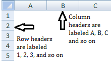
By default, the row and column headers are displayed. It displays letters for indicating columns and numbers for indicating the rows. It helps to enter the data into the specific cells). Also, if cell(s) are selected then the row and column headers get shaded to indicate the selected cells. If you decide to hide the row and column headers then you may do so by changing an Excel option. You may also turn on this option later. Perform the following steps to show or hide row and column headers:
1. Open Microsoft Excel.
2. Click the Microsoft Office Button and click Excel Options.
3. From the Excel Options dialog box, click Advanced from the left pane.
4. From the right pane, scroll down to the Display options for this worksheet: and do one of the following:
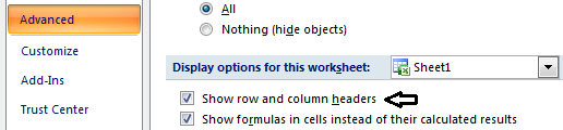
To show the row and column headers - Click to place a checkmark besides Show row and column headers.
To hide the row and column headers - Click to remove the checkmark besides Show row and column headers.
5. Click OK.

Change the direction of the Enter key in Excel 2007

In Excel 2007, when you enter data into a cell and press the TAB or ENTER key then the cell that is to the right becomes the active cell. You can change this behavior by changing an Excel option and make the cell that is to the left or top or bottom to become the active cell.
Please note that this setting cannot be done for the TAB key. Pressing the TAB key will always move to the right. Perform the following steps to change the direction of the ENTER key:
1. Open Microsoft Excel.
2. Click the Microsoft Office Button and click Excel Options.
3. From the Excel Options dialog box, click Advanced from the left pane.
4. From the right pane, under Editing options, click to place a checkmark besides After pressing Enter, move selection. Click the direction in the Direction box.
5. Click OK.

Enable or disable editing directly in cells in Excel 2007

By default, you can edit directly in cells. You can enable or disable editing directly in cells by changing an Excel option. Perform the following steps to do so:
1. Open Microsoft Excel.
2. Click the Microsoft Office Button and click Excel Options.
3. From the Excel Options dialog box, click Advanced from the left pane.
4. From the right pane, under Editing options, do one of the following:
a. To edit directly in cells: Click to place a check mark besides Allow editing directly in cells.
b. To disable editing directly in cells: Click to remove the check mark besides Allow editing directly in cells.
5. Click OK.

Display or hide the fill handle in Excel 2007

By default, Excel displays the fill handle. You can display or hide the fill handle by performing the following steps:
1. Open Microsoft Excel.
2. Click the Microsoft Office Button and click Excel Options.
3. From the Excel Options dialog box, click Advanced from the left pane.
4. From the right pane, under Editing options, do one of the following:
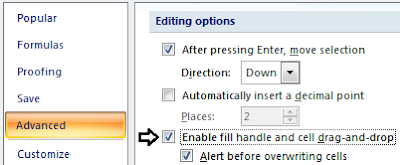
a. To display the fill handle: Click to     place a check mark besides Enable fill handle and cell drag-and-drop.
b. To hide the fill handle: Click to remove the check mark besides Enable fill handle and cell drag-and-drop.
5. Click OK.

Unable to drag page breaks in Page Break Preview in Excel 2007

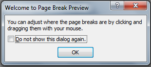
When you try to adjust the page breaks, you see the Welcome to Page Break Preview dialog box that says You can adjust where the page breaks are by clicking and dragging them with your mouse. You click OK but you are unable to adjust the page breaks.

The cause for this is the Enable fill handle and cell drag-and-drop check box is cleared. Perform the following to check the Enable fill handle and cell drag-and-drop check box so as to drag page breaks in Page Break Preview:

1. Open Microsoft Excel.
2. Click the Microsoft Office Button and click Excel Options.
3. From the Excel Options dialog box, click Advanced from the left pane.
4. From the right pane, under Editing options, click to place a check mark besides Enable fill handle and cell drag-and-drop.
5. Click OK.

Show or hide row and column headers in Excel 2007

The rows and columns in a worksheet display the headers by default. The column headers start with text (A, B, C, and so on). The row headers start with numbers (1, 2, 3, and so on). You can hide the headers to add extra space or you can show the headers.

Perform the following steps to show or hide the row and column headers:
1. Open Microsoft Excel.
2. Click the Microsoft Office Button and click Excel Options.
3. From the Excel Options dialog box, click Advanced from the left pane.
4. From the right pane, under Display options for this worksheet:, do one of the following:
To show row and column headers: Click to place a checkmark besides Show row and column headers.
To hide row and column headers: Click to remove the checkmark besides Show row and column headers.
5. Click OK.

Note:
The steps provided above applies at the worksheet level. You can select multiple sheets to change the setting at the same time.

Show or hide formulas in Excel 2007

When a formula is entered in a cell, the calculated result is displayed in the cell and the formula is displayed in the Formula Bar. If you want to avoid others from seeing the formulas then you choose to hide the formulas. You can hide the formulas by hiding the Formula Bar or by protecting the worksheet and making selections from the Format Cells dialog box or by toggling using the Show Formulas command on the Ribbon. See the following for information related to this.

Show or hide the Formula Bar:
1. Open Microsoft Excel.
2. Click the Microsoft Office Button and click Excel Options.
3. From the Excel Options dialog box, click Advanced from the left pane.
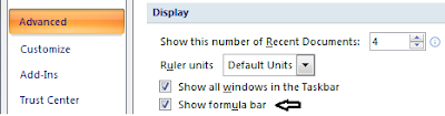
4. From the right pane: scroll down, under Display, do one of the following:
    To show the Formula Bar: Click to place a checkmark besides Show formula bar.
    To hide the Formula Bar: Click to remove the checkmark besides Show formula bar.
5. Click OK.

Show or hide formulas from Format Cells dialog box and protecting the worksheet:
1. Select the cell(s) that has the formulas. For selecting multiple cells, click the first cell and then press the CTRL key. Keep the CTRL key in pressed state and select other cells.
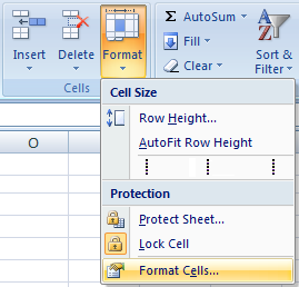
2. On the Home tab, in the Cells group, click Format and click Format Cells...

3. From the Format Cells dialog box, click the Protection tab, do one of the following:
    To hide the formulas: Click to place the checkmark besides Locked and Hidden.
    To show the formulas: Click to remove the checkmark besides Hidden.

4. Click OK.
5. On the Review tab, in the Changes group, click Protect Sheet.
6. From the Protect Sheet dialog box, assign a password or leave it blank and click OK.

Toggling using the Show Formulas command on the Ribbon
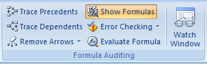
By default, the calculated result appears in a cell that has a formula. You can toggle by displaying the formula in the cell or the calculated value. To do this, click the Formulas tab. On the Formula Auditing group, click Show Formulas.

Show or hide Formula Bar in Excel 2007

The contents in an active cell get displayed in the Formula Bar and is placed just below the Ribbon. The Formula Bar displays text, number or data exactly as it is entered in a cell. What if you entered a formula in a cell. The answer is, the calculated value is displayed in the cell and the formula is displayed in the Formula Bar.
For some reasons if you decide to hide the formulas then one of the ways to do is to hide the Formula Bar. This action is reversible and you can view the Formula Bar if it is hidden. Perform the following steps to show or hide the Formula Bar:
1. Open Microsoft Excel.
2. Click the Microsoft Office Button and click Excel Options.
3. From the Excel Options dialog box, click Advanced from the left pane.
4. From the right pane: scroll down, under Display, do one of the following:
   To show the Formula Bar: Click to place a checkmark besides Show formula bar.
   To hide the Formula Bar: Click to remove the checkmark besides Show formula bar.
5. Click OK.

Clear the list of Recent Documents in Excel 2007

In Excel 2007, by default 17 documents are listed under Recent Documents. You can change this number to a value ranging from 0 to 50. If you had entered zero then the list is cleared and no recent files will be displayed under Recent Documents. Perform the following steps to clear the list of Recent Documents:

1. Open Microsoft Excel.
2. Click the Microsoft Office Button and click Excel Options.
3. From the Excel Options dialog box, click Advanced from the left pane.
4. From the right pane, under Display, enter 0 in the Show this number of Recent Documents: box.
5. Click OK.

Change the number of Recent Documents in Excel 2007

When you click the Microsoft Office Button , you will see New, Open, Save, Save As and so on. To the right, you will use the files that you recently opened under the Recent Documents list. By default, 17 files are displayed. You can change this number to a value from 0 to 50. To change the number of Recent Documents, perform the following steps:

1. Open Microsoft Excel.
2. Click the Microsoft Office Button and click Excel Options.
3. From the Excel Options dialog box, click Advanced from the left pane.
4. From the right pane, under Display, enter a value from 0 to 50 in the Show this number of Recent Documents: box or click the UP arrow or DOWN arrow buttons to increase or decrease the number of files.
5. Click OK.

Note:
If 0 is entered in the Show this number of Recent Documents: box then you will have no files displayed under Recent Documents.

Show or hide vertical scroll bar in Excel 2007

By default the vertical scroll bar appears even if you open a blank workbook. If your worksheet has a large data then the horizontal scroll bar will help you to scroll up or down. If you feel comfortable navigating in the worksheet through keyboard then you may hide the vertical scrollbar. This action can be reversed and you can make the vertical scrollbar visible whenever needed by perform the following steps:
1. Open Microsoft Excel.
2. Click the Microsoft Office Button and click Excel Options.
3. From the Excel Options dialog box, click Advanced from the left pane.
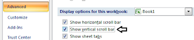
4. From the right pane, under Display options for this workbook:, do one of the following:
    To show the vertical scroll bar: Click to place a checkmark besides Show vertical scroll bar.
    To hide the vertical scroll bar: Click to remove the checkmark besides Show vertical scroll bar.
5. Click OK.

Note:
The setting applies to the entire workbook.

Show or hide horizontal scroll bar in Excel 2007

By default the horizontal scroll bar appears even if you open a blank workbook. If your worksheet has a large data then the horizontal scroll bar will help you to scroll to the right or left. If you feel comfortable navigating in the worksheet through keyboard then you may hide the horizontal scrollbar. This action can be reversed and you can make the horizontal scrollbar visible whenever needed by perform the following steps:
1. Open Microsoft Excel.
2. Click the Microsoft Office Button and click Excel Options.
3. From the Excel Options dialog box, click Advanced from the left pane.
4. From the right pane, under Display options for this workbook:, do one of the following:
    To show the horizontal scroll bar: Click to place a checkmark besides Show horizontal scroll bar.
    To hide the horizontal scroll bar: Click to remove the checkmark besides Show horizontal scroll bar.
5. Click OK.

Note:
The setting applies to the entire workbook.

Display or hide sheet tabs in Excel 2007

By default, Excel 2007 displays the sheet tabs. Sheet tabs are placed just above the status bar and help to easily move around the worksheets. You have the option to show or hide the sheet tabs for a particular workbook. Perform the following to do so:
1. Open Microsoft Excel.
2. Click the Microsoft Office Button and click Excel Options.
3. From the Excel Options dialog box, click Advanced from the left pane.
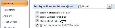
4. From the right pane, under Display options for this workbook:, do one of the following:
     a. To display the sheet tabs, click to place a checkmark besides Show sheet tabs.
     b. To hide the sheet tabs, click to remove the checkmark besides Show sheet tabs.
5. Click OK.

Change the gridline color in Excel 2007

You can customize the look of the worksheet by applying a different color to the gridlines. You can change the gridline for a single worksheet or you can select multiple worksheets and change the gridlines color at the same time. To select multiple worksheets do the following:
Selecting all worksheets: Right click on the sheet tab and click Select All Sheets.
Selecting adjacent worksheets: Click on a sheet tab and then press the Shift key. Keep the Shift key in pressed state, click to select the last worksheet.
Selecting non-adjacent worksheets: Click on a sheet tab and then press the Ctrl key. Keep the Ctrl key in pressed state, click to select other worksheets.

Once the selection of the worksheet(s) is over, perform the following steps to change the gridline color:
1. Open Microsoft Excel.
2. Click the Microsoft Office Button and click Excel Options.

3. From the Excel Options dialog box, click Advanced from the left pane.

4. From the right pane, scroll the list. Under Display options for this worksheet: make sure that the Show gridlines is checked. Click the Gridline color box and select a color.

5. Click OK.

Change the default file location in Excel 2007

In Excel 2007, when you save a file for the first time by clicking the Save command that is present in the Quick Access Toolbar or by pressing Ctrl + S then Excel 2007 saves the file in the following location.

In Windows XP the location is C:\Documents and Settings\username\My Documents
In Windows Vista and Windows 7 the location is C:\Users\ username\Documents

You can change the location by performing the following steps:
1. Open Microsoft Excel.
2. Click the Microsoft Office Button and click Excel Options.
3. From the Excel Options dialog box, click Save from the left pane.
4. From the right pane, under Save workbooks, specify a location in the Default file location: box.
5. Click OK.

Show or hide gridlines on a worksheet in Excel 2007

By default, Excel 2007 displays lines around cells. These lines are called gridlines. You can select a single worksheet to make the gridlines visible or hidden (or) you can select multiple sheets and make the gridlines visible or hidden at the same time. To select multiple worksheets do the following:
Selecting all worksheets: Right click on the sheet tab and click Select All Sheets.
Or
Selecting adjacent worksheets: Click on a worksheet and then press the Shift key. Keep the Shift key in pressed state, click to select the last worksheet.
Or
Selecting non-adjacent worksheets: Click on a worksheet and then press the Ctrl key. Keep the Ctrl key in pressed state, click to select other worksheets.

Once the selection of the worksheet(s) is over, perform the following steps to hide the gridlines:
1. Open the workbook and click on the worksheet(s).
2. Click View tab. In the Show/Hide group, click to clear the checkmark besides Gridlines.

You can also hide the gridlines from the Excel Options dialog box. The steps are:
1. Click the Microsoft Office Button and click Excel Options.
2. From the Excel Options dialog box, click Advanced from the left pane.
3. From the right pane, scroll down to the Display options for this worksheet section and click to remove the checkmark besides Show gridlines.
4. Click OK.

To show the gridlines click the View tab, in the Show/Hide group click to place the checkmark besides Gridlines.

Show or hide the display of zero values in Excel 2007

Excel 2007 displays zero values in cells by default. You can customize and have Microsoft Excel display blank cell(s) when the value zero is in the cell(s). Perform the following steps to hide the display of zero values:
1. Open Microsoft Excel.
2. Click the Microsoft Office Button and click Excel Options.
3. From the Excel Options dialog box, click Advanced from the left pane.
4. From the right pane, scroll down to the Display options for this worksheet: section. Click to remove the checkmark besides Show a zero in cells that have zero value.
5. Click OK.

To show the zero value, repeat the above steps and click to place the checkmark besides Show a zero in cells that have zero value in step 4.

Note:
The option of showing or hiding the zero values applies only to the selected worksheet and not to the entire workbook.