Freeze Panes in Excel 2007

If you are working with large worksheets that has headings in rows or columns and if you scroll down or across the worksheet, the headings will not be visible. To make the headings visible at all time, Excel allows you to freeze panes to lock rows and columns. You have the options of freezing the top row, top column or freezing multiple rows and/or columns. 

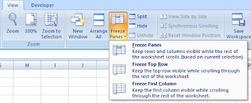
Freeze top row:
On the View tab, in the Window group click Freeze Panes and click Freeze Top Row.

Freeze top column:
On the View tab, in the Window group click Freeze Panes and click Freeze Top Column.

Freeze multiple rows and/or columns:
To freeze multiple rows, say 3 rows, click the first cell on the fourth row (cell A4). On the View tab, in the Window group click Freeze Panes and click Freeze Panes.
In general to freeze 'n' rows, click on the first cell in the 'n+1' row and perform the above procedure.

The same applies if you want to freeze multiple columns. For example, to freeze 2 columns, click on the first cell in the 3rd column (cell C1). On the View tab, in the Window group click Freeze Panes and click Freeze Panes.

To freeze multiple rows and multiple columns, say if you want to freeze 2 rows and 3 columns, click the cell below 2nd row and to the right of 3rd column, which in our case is the cell D3. In general to freeze x number of rows and y number of columns, move to the cell that is x+1 number towards right and y+1 number below.